

Richard Jerousek and I.
He is in love with Saturn’s Rings
A short Research Biography ( For ML People)
A bit of technical background: I am an AI research scientist, I worked on a variety of areas, from theory to practice and applications of AI. On implementations, I worked from Cuda level ambitions of changing the Conv layer, to creating ordered statistics on pooling layers, to implementing probabilistic auto-differentiation platforms. Here, this was my self promotion.
I failed my statistics course in undergrad, but somehow I ended up deeply in Probability Theory and Information Theory in my studies. Another one of those academia stories. I didn’t choose to study AI, it just grew on me. At some point, I formed an unhealthy obsession toward interpreting even viruses as torn pieces of a book called “Torn papers from the book called “The celestial condition of planet earth” ”. But I guess it was the question of unknownness that really dragged me there.
In AI, one of my dearest research path was on compression of bit string, for inference.I researched that for a while, the premise was to look at collection of bitstrings, and constructing invertible boolean functions that makes the bits statistically independent. And to do that, the question is to find an invertible function on the bitstrings so that the sum of marginal entropies decreases. Meaning the entropy of the first bit plus the entropy of the second bit and so on decreases when the bits become independent.
I worked on that, and I realized the curse of dimensionality in the binary case. I could compress but couldn’t generalize But now I know better, all hope is not lost. What was the missing ingredient? Regularization or Forgetting.
I moved from that project to a parallel, i was working on discreteness in neural network, not to threshold values, but to interpret values as unnormalized log-probabilities on finite number of states, and It lead to this paper, Rediscovering CNNs Through Classification of Finite State Distributions. Again in hindsight, I dont fully approve of the approach discussed in the paper. I think it is a valuable starting point, to get out of the curse of dimensionality, already existing even in a single real number scalar value, the uncountable infinity.
Idealogically now, I prefer exponentially large but finite states to work with theoretically, than to get lost in the uncountable infinity of real numbers with the hope of locality and smoothness. I dont have anything against smoothness though, I can interpret it in the sense of forgetting. Number 4.2432 is not a point, its a region, because we missed the infinite 0’s. And in calculus class, every teacher, with a marker, shows a point, on the white board, with a region, as thick as the marker.
Working on finite state representations, I started experimenting using only probabilistic binary variables inside of CNNs, and derived the way to optimize the probability distributions governing the binary random variables. As expected the problem of sampling from conditional distributions makes the optimization very slow, but there are turn arounds that I will eventually write in more details in this website. At the time, I had so many parallel interests and research, and one of them was the question of Priors, and Edwin T Jaynes, was someone that influenced me from beginning of my research. The consistent issue that I faced, in optimizing probabilistic systems, was that the probability distribution of hidden variables, would tend to degeneracy, and the optimization stops. This problem could’ve been caused, either by incompleteness of the model family, meaning the model was not a universal approximator, or the regularization.
So there should have been a way to resolve that. In parallel “the prior” research helped me.
I remember 2015, I was talking to George, I call him my applied mathematics professor, about Rejection Sampling, and I was wondering what would be the distribution of rejected samples, just to play. And I eventually wrote a report, that was basically finding the distribution of the rejected samples, and I called it the complement distribution. And I thought that was the interesting finding, but it was the rate of rejection that was interesting.
So facing my optimization problem, and having that research somewhere in the cabinet of the thought, one day I realized, 1 - (rejection rate) is the probability of the model itself. So I revisted that, and with that line of thought Maximum Probability Theorem, as a name, was born to me.
I remember I was so happy that I ran to Alireza’s lab, my research buddy, and I told him about my finding which was the review of probabilistic machine learning. Where models are sets, and they have a probability mass, not density, no matter what the parameterization is. And that moment or maybe a day later, I remember I was thinking about all the time, that I smoked my cigarettes, at the staircase behind the department, and my head was painfully steaming, thinking in loops of what would be the prior over parameters of a model, and finally I have found a direction to it.
MPT, gives a systematic view to regularize models. Look, when we are working with complex models, of course we cant say minimizing the norm of parameter vectors, are not necessarily regulating the behaviour of the model. We needed to come up with a black box regularization. MPT does that. MPT simply comes in as a term in the objective function. And I showed in an empirical study ( Link ) of 1000 networks , doing black box regularization on models, consistently increases the average accuracy of models with randomized hyper parameters as well as reducing the variance of the accuracy on the test set.
That is maybe a flavor of how I romanticized research. In summary, I have worked on generalization, optimization and model building. and to this day, I think, there is a way to look at bitstrings, and there is hope to use our computation efficiently. Or to stop deploying AI so fast, and before realizing at least some rigor about generalization. Not approximating bounds, but finding what is the best we could do for a guarantee. And also appreciate the subjectivity that is induced in any algorithm, usually on a complex society. And to understand where to use this machinery and where not to. We should’ve learnt some lessons from testing The Bomb in the atmosphere. And Maybe the solution to our untamed rational is out there, maybe someone wrote an article that is missed in the academic publication industry. I hope to see that some day.
At this point, its tiring for me to say what was the full story of my research but briefly I will say, that after MPT, and models, my interest went directly to question of generalization. Generalization heavily relates to regularization, and I started formalizing this relation. Its actually not that hard. If your model is sensitive to change of input locally, it means that in the parameter space, perturbation of training data, will change the loss drastically. And imagine you choose a parameterization, that is sensitive to fluctuation in the input data. Of course, the variation between training and test data, will change the loss. That is why, we like smooth functions. Now this is an entrance into the generalization question. I love to get back to these sorts of problems that are important in future of AI, but neither academia nor industry seem to have time for it.
Now to lighten the mood I brought one of my most comic ground breaking findings
Info Theory Entertainment: How to Classify Images, Using Only Mouse and Windows 98
This is a comic demo of my obsession with information theory.
Gather a training set of Cat images, and dog images. Create a folder called cats, and create a folder called dogs.
Put all cat images in the cat folder, put all the dog images in the dog folder. right click on the folders and send both to compress format using say ZIP. right click on the zip files, write down the size of each zipped folder.
When test image comes in, put the image in the cat folder, zip it, find how much the size of the zip file increases. do the same with the dog folder. whichever zip file that has the least increased size, it is the predicted class.
And In my spare time, I tried it on CIFAR 10. it has an accuracy of 15 percent. which was amazing for me :) If you are familiar with ZIP algorithm and the window sizes in Lempel Ziv like algorithms, you can see why 15 percent is surprisingly good for image data.
The Main Theory:
In AI, we have three problems, no matter what the task is. Language is discrete and factorized input data, or vision, which is a quantized continuous series of observed variables, or regression, which is a way of telling our selves the input and output is continuous,
The three problems that I present is the following
1. Completeness: What is the schema of a model with arbitrary number of variables, that can approximate relation of input and output for any type of input and output.
2. Generalization: How to train a complete model that works on unseen data, what is the angle that we can generalize to unseen observations - spoiler alert: there is an angle
3. Optimization: How to guarantee that a complete model can be optimized without looking at the data before hand, or having a knowledge of scale of variables.
First lets just say, Enough with continous variables. At the end of the day, in a computer, the data is digitized. In digital data, the scale, is the dimension. The norm is reflected in the number of bits
An umbrella overview and the reduction: Its all about coin flips
The entirety of the problem of statistical inference boils down to coin flips or roll of dice.
Consider the classification problem. The classification problem on finite digits, is inferring, digits from input digits.
Now if we concatenate the input and the output, we can say, the problem is finding a joint distribution on input and output. Having the joint distribution on input and output we can condition on the input and infer the output. Lets say we have N bits for input, and M bits for output. we have 2^(N+M) side die, that we roll multiple times and we want to find the joint distribution. Of course, that when we have die of 1000000 side, 5 rolls does not tell us anything about the die. So what do we do? We factorize.
We can think of of 100000 side die, as combination of Log(100000) number of dice being thrown, and we can now have hopes in finding the marginal distribution of each die with few samples. In theory we assumed independence of the die ( or better I say, under null hypothesis, did not assume relation). Now whether we are looking at completion of a sentence, translation of language, classification of images, segmentation, etc, we are looking at coin flips, our die has 2 sides.
Now simmetrically, the question of finding a Joint distribution reduces, to the problem of classification. Does this sequence of dice rolls come from our distirubtion or not. Under a prior for input and output, if for each sequence of input and output we have the probability of whether this sequence belongs to our distribution or not, we can generate samples from the distribution. In essence, the problem of classification and finding a joint distribution are equivalent. This is similar to the Set formalization aspect, we can have a membership function for the set, or have a generator of the set.
So I ask this question:
Why do we focus on continuous random variables? and then for efficiency quantize?
Lets go Full Digital.
A Note on Completeness:
The Model Cannot be Feasibly Complete
If you look at how we determine a membership function, we know one thing. for N variables of say 2 states, i.e. coins, If we write down the logic table of a membership function, we need exactly 2^N variables. So for a model operating on 100 bits, we need 2^100 bits to represent possible relations. Now if we go probabilistic, in a determinsitic computer, and to define a probability distribution over 100 bits, we need 2^100 - 1 real valued parameters. You know its not feasible. So we are at square one, Factorization. We can always factorize in this way or that way. Thats how Convolution or Lempel Ziv works. It factorizes the input data and as you factorize your number of observation increases.
Regularization The Key to Generalization:
Consider the following optimization landscape.
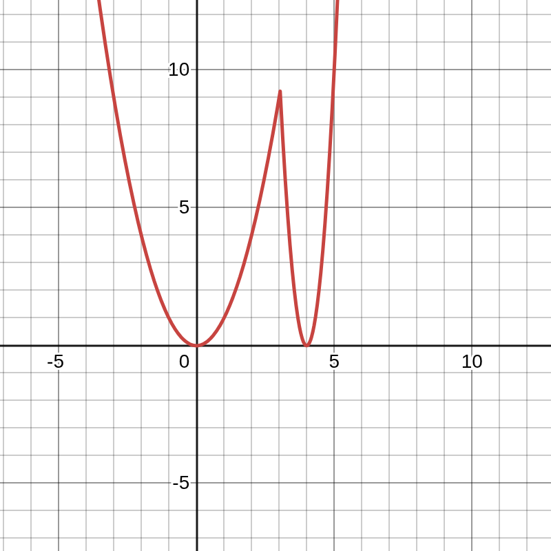
Which local optimum is preferable?
Realistically, this loss function is a function of parameters as well as the training data. The wideness of the solution is an indicator of whether the solution is sensitive to perturbation of the training data. we know that the optimum parameter is a function of the training data, and if the rate of change of the optimum parameter configuration with respect to training data is large, we can say that changing the training to test data will shift the optimum parameter. So here is the angle, the wider the better. The wider optimum in terms of input data and the parameters is preferable.
The Angle to Generalization is Indifference
Regularization of models, from a deterministic perspective, is smoothing the output of the function with respect to input. Smoothing means, that given a topology of space, variation of input would not cause extreme variation in the output. For example, in CNNs, it is said that we prefer parameterizations with smaller norm. The reason for this, is that CNNs are not that black box after all, we know the parameters mostly represent the parameters of linear transformations. There is no magic in an L2 regualrization or L1 Regularization, both are imagination of a space of parameters, under which we prefer small normed parameter vectors.
With small normed vector, the magnitude of the gradient of the output with respect to input tends to be less. Making the CNN more smooth. Now how do we formalize this? How do we go full black box.
Assume You Know Nothing About the Black Box
We could have the norm of the gradient of the output to input as the regularizing factor, but if you have hands on experience with numerical evaluations, we need second order derivatives, and it is computationally expensive. Or we can look at the problem probabilistically. But before that, let me explain a finding.
What is probability?
What is probability?
is it something that we can measure? Is it observable?
No
Probability is a measure of size, for us to formalize what is out knowledge and uncertainty, but as soon as anything is measured or realized, probability goes out the window.
What is a model?
In probability, we often look at the model as a device with some parameters and some priors on them. The device is fixed and the parameters are changing. The device dictates the relation of the parameters to the likelihood of observable outcome. Now, Take a look at a model for a flawed coin. We have two observable outcomes, and a continuous parameter. Say the ratio of probability of Head vs Tail, i.e. Theta = P(Head)/ P(Tail)
Now, the convention is, to have a model of the coin, we set a prior over the parameter. In this case, for two observable outcomes, we need to scratch our head pretty hard, to look for a suitable prior, in the pool of uncountable infinite possibilities, for the parameter.
Something is not right.
But What if ….
What if we define models as sets…
When Kolmogorov formalized probability theory, what was most fascinating, was the deterministic nature of the formalization. Now lets take a look at Kolmogorov’s formalization
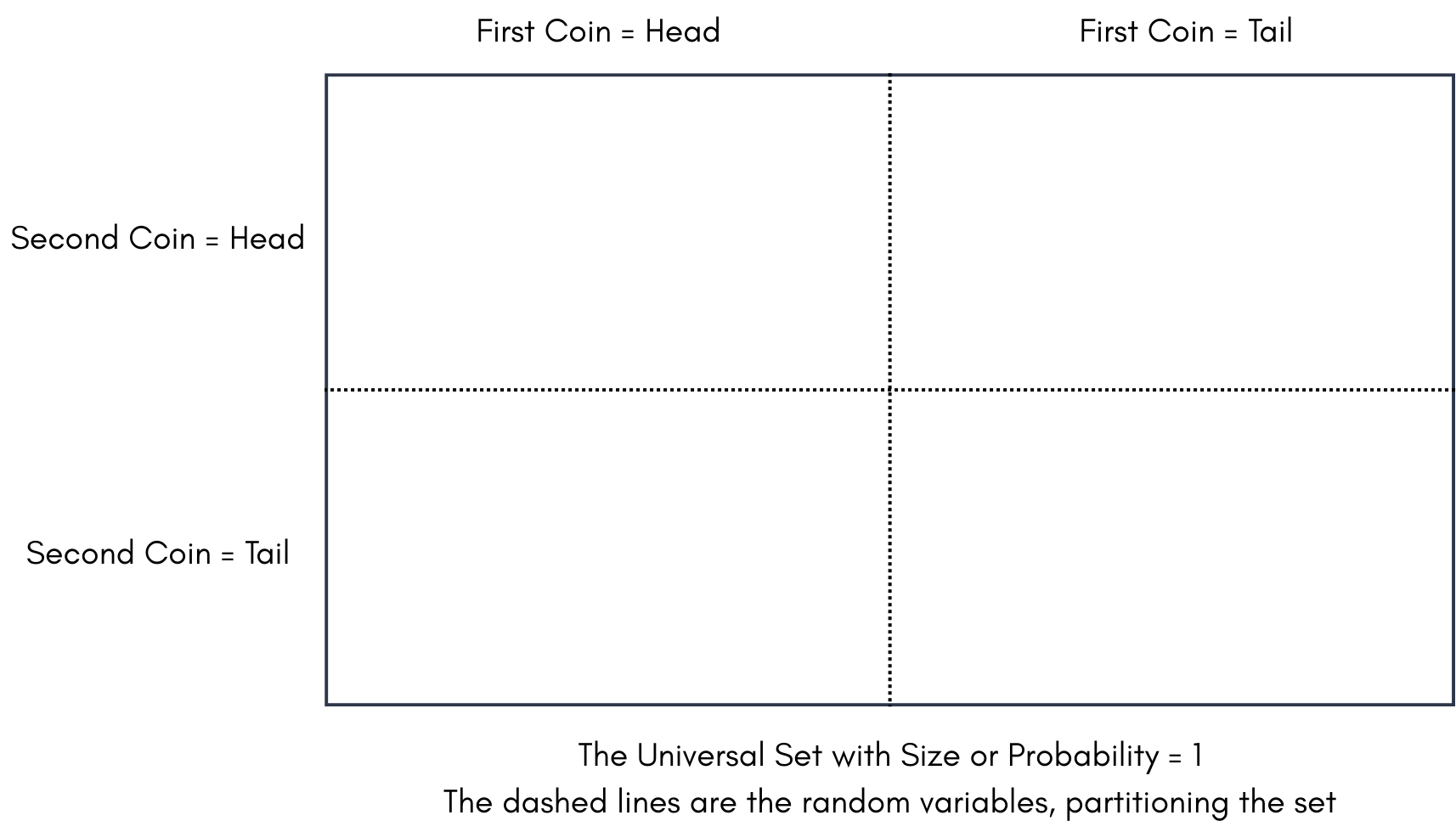
In above figure, The probability space is the box you see. The size of the box ( e.g. Area) is 1. Or in other words the probability of the Box is 1. or in yet other words, the probability of any event being part of the box is 1. The dashed lines are the random variables, for example fate of a coin. The coin separates the box into two parts, Head and Tail. Now this box represents our prior, if the coin equally splits the box into two parts, we have a uniform prior over the outcome of the coin flip.
Now how do we formalize, a flawed coin? say we learnt something about the coin, and we now know there is more of a chance of Heads than Tails. How do we show that? Do we Redraw the box? or create a random variable called probability of Head, and partition this space into uncountably infinite partitions.
Can you believe this simple picture took me 5 years?
And Even now I know why it took me so long.
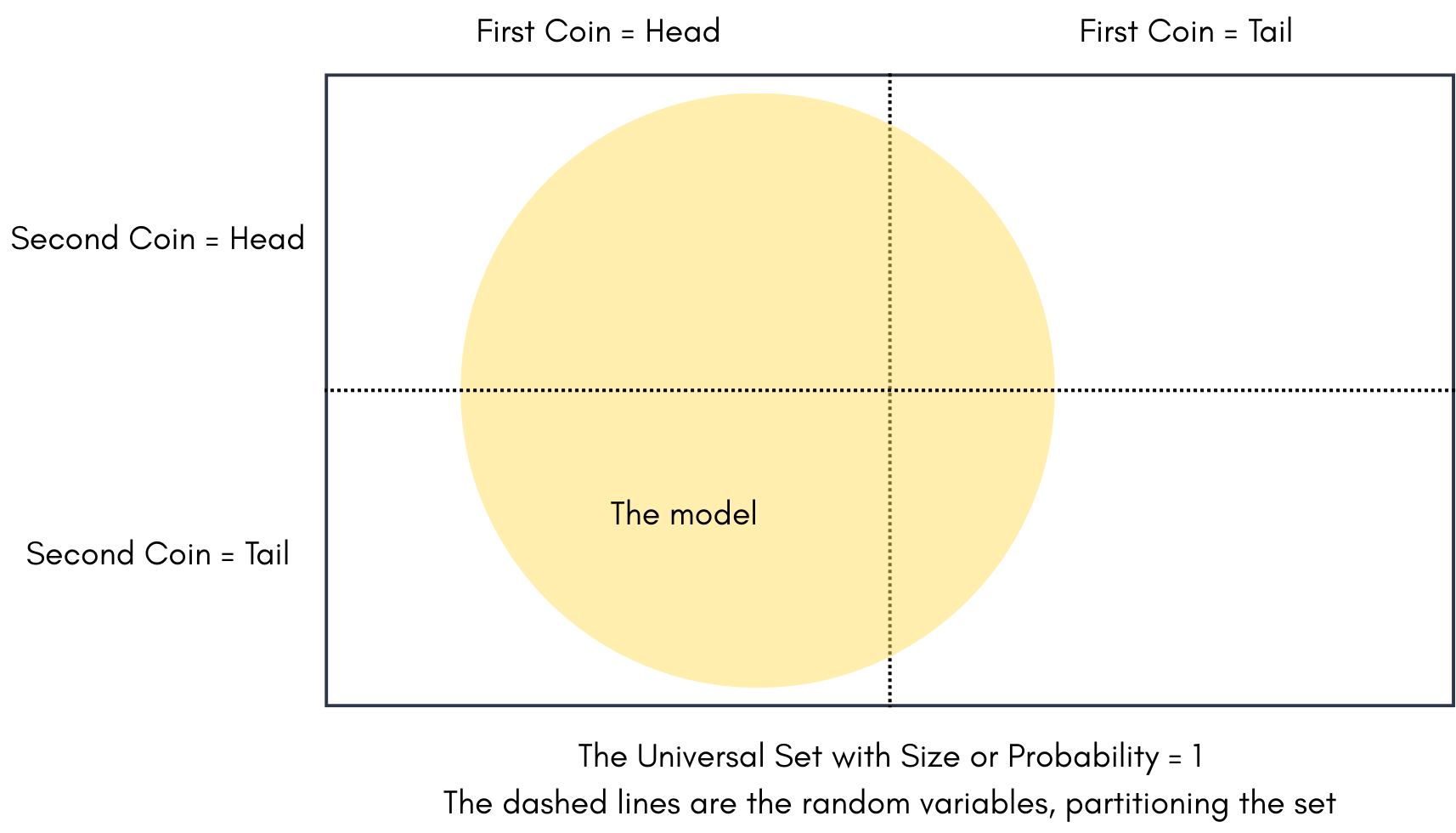
No we can simply define the model as a set. Above the yellow circle becomes a model.
Is the area of the First coin=Head and First Coin=Tail in the yellow circle equal? Of course Not. There we go, now we can define any probability distribution on our random variables by drawing subsets.
What is the area of a model, if we know the probability distribution that it imposes on the coin or any random variable?
We have an upper bound for it. Try to enlarge the circle so that the proportions of the area of coin being head and tail is maintained. The area cannot be 1, if the proportation of the partitions is not equal. of course in a uniform prior example. Maximum Probability Theorem calculates this upperbound.
Now Here is Maximum Probability Theorem:
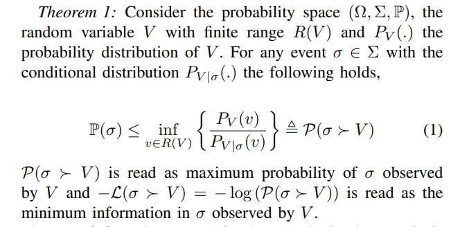
To be continued, Author at work ….